A probe at layer 0 is a lie detector for your experiment
The result that should have worried me
I trained a linear probe to read sentiment off Gemma 3 1B, and it classified every held-out example correctly. Not at the layer I expected, where the model has had a chance to think, but at layer 0: the raw input embedding, before a single attention head or MLP has run. Held-out accuracy was 1.000 at the embedding, and stayed pinned at 1.000 across almost all of the model’s 26 layers (27 residual readout points, counting the embedding).
That is not a win. That is the probe reading the dictionary.
The interesting object in interpretability is rarely the accuracy number. It is the accuracy-by-layer curve: how separability of a concept changes as you move up the residual stream. A flat line at the ceiling from layer 0 onward is a particular and unflattering shape. It says the concept was linearly present in the input and the transformer did not need to build it. I learned that my apparatus works and that sentiment is linearly decodable. I did not learn anything about where the model computes sentiment, because on this task it does not have to.
This post is about that failure and the fix: a second probe, same model, same method, same 100% ceiling, that tells the truth about where a concept forms. The two curves look almost identical at the top and mean opposite things.
Probing in one paragraph
A linear probe is a logistic-regression classifier trained on a model’s internal activations to predict some label (here, sentiment). You fit one probe per layer, on a train split, and score it on held-out prompts. Plotting probe accuracy against layer is the oldest diagnostic in the interpretability toolbox (Alain & Bengio, 2016): it asks at what depth does this concept become linearly readable? The whole method rests on a linear-representation assumption, that high-level concepts live as directions in activation space (Park, Choe & Veitch, 2024). The probe finds the direction; the curve tells you when it shows up.
The catch, well documented (Belinkov, 2022), is that a probe can score high for boring reasons. It might be reading a lexical artifact rather than a computed feature, or it might just have enough capacity to fit noise. So you bring controls. I used a vocabulary-disjoint train/test split (held-out sentiment words never appear in training) and a shuffled-label control: retrain the same-capacity probe on permuted labels, and report selectivity, real accuracy minus control accuracy (Hewitt & Liang, 2019). High accuracy with near-zero selectivity is the probe’s capacity talking, not the model’s representation.
Experiment A: sentiment, the easy way
The first concept was plain sentiment: positive versus negative adjectives in fixed templates, 144 training prompts and 48 held-out, balanced. The vocab-disjoint split meant the probe could not memorise specific words. Here is what the curve did.
The red curve in the figure below is flat at 1.000 from layer 0, dipping only slightly (to about 0.96-0.98) in the deepest layers. Best layer: 0. Selectivity is high too, peaking 0.73 at layer 3, so this is not the probe fitting noise; the signal is real. It is just real in the wrong place.
A vocab-disjoint split blocks one shortcut (memorising the exact held-out words) but not a subtler one: held-out positive adjectives still sit near training positives in embedding space. “Glorious” and “wonderful” are different tokens but neighbours as vectors. The probe does not need the transformer to separate them; the embedding already has. A flat-at-ceiling curve from layer 0 is the signature of a concept that is present in the input, not constructed by the model. The honest read of Experiment A is a cautionary one, which is exactly why it is worth reporting.
Experiment B: make the label impossible to look up
The fix is to choose a concept whose label cannot be read off any single word. I used negation-composed sentiment: the label is
\[\text{net sentiment} = \text{adjective polarity} \;\oplus\; \text{negation}\]
an exclusive-or. “Wonderful” is positive; “not wonderful” is negative; “terrible” is negative; “not terrible” is positive. Now the adjective alone tells you nothing, because both classes contain both polarities, and the negation alone tells you nothing either. You have to compose the two. A linear model over token identities (a bag-of-tokens baseline) provably cannot represent XOR, and indeed it scores at chance. 192 training prompts, 64 held-out.
This is the same move a good measurement pipeline makes in any setting with an obvious shortcut: choose a contrast where the shortcut cancels before asking the model what it computed.
The blue curve is the payoff. Layer 0, the embedding: 0.500, exactly chance. The composed concept is simply not there in the input. Then it climbs, layer by layer, 0.59, 0.64, 0.56, 0.73, 0.88, 0.97, 0.98, and reaches the ceiling of 1.000 by layer 8, where it plateaus for the rest of the stack. The shuffled control stays near chance throughout, so the rise is representation, not capacity.
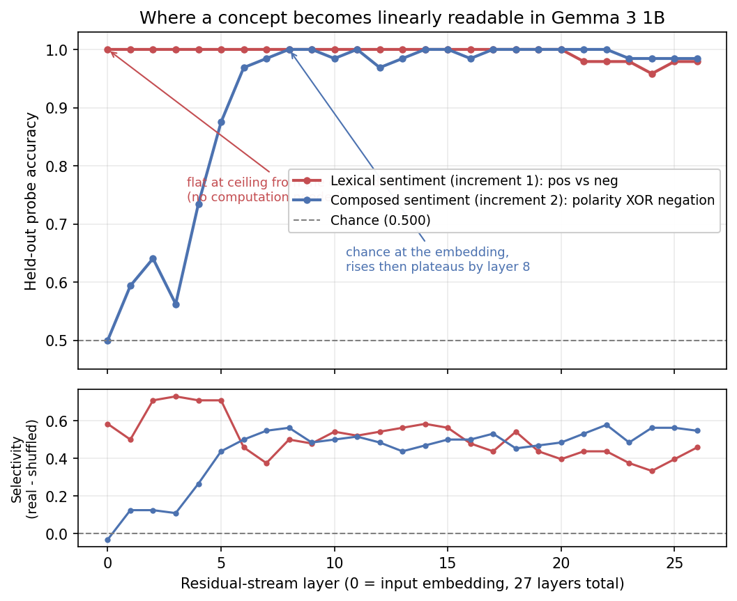
Same model, same probe, same ceiling at the top. The red curve was born at 1.000; the blue curve had to be built to 1.000. That rising flank, layers 1 through 8, is the depth interval where Gemma 3 1B reorganises its geometry to make the composed concept linearly separable. Recent work calls this a concept’s allocation zone, the contiguous region of depth where a concept forms rather than the single layer where it peaks (Henry, 2026). Experiment A has no allocation zone inside the transformer; the concept arrives pre-allocated. Experiment B’s allocation zone is the early-to- mid stack.
What this does not show
The temptation now is to say “the model computes negation at layer 8.” I have not earned that, and the same caution that makes Experiment A honest applies here.
- This is a readout, not a localisation. A linear probe on a mean-pooled residual tells you when the composed direction becomes linearly readable by this probe, not which heads or MLPs assemble it. “Readable by layer 8” is the ceiling of this particular readout, not a claim about the only place the information lives.
- The best layer is a snapshot, not the process. Reporting “best layer 8” hides that separability is built across a whole region, and separation curves are often multimodal with subtle but causally active structure outside the obvious peak (Henry, 2026). The plateau after layer 8 does not mean nothing else happens there.
- The plateau is at 1.000. The concept is still comfortably separable, so this design cannot measure a margin; a harder or noisier composed concept would.
Localising the mechanism, which heads move the negated representation and where the composition actually happens, is a causal-intervention question (activation patching), and it is the next experiment. This post is deliberately the readout result, because the readout is already enough to make one clean point: the accuracy number lied in Experiment A and told the truth in Experiment B, and the only way to tell which was to look at the shape.
The same confound, in a different signal
This pattern is not specific to transformers. A linear decoder can succeed for a reason upstream of the target mechanism: a shortcut feature, an artifact, or a background variable that happens to correlate with the label. The decoder is real; the accuracy is real; the interpretation is wrong. The fix is to close the trivial route by design, then ask whether the decoder still works.
A probe at layer 0 is that diagnostic in transformer form. It catches the case where the classifier is reading the input representation rather than the model’s computation. For this kind of probing, I now trust the shape of the depth curve more than the best-layer number. The XOR redesign forces the model to actually combine two pieces of information, so when the probe succeeds, the success is about something the model had to build.
What this taught me
- The number is not the finding; the curve is. Two probes hit 1.000 and meant opposite things. Best-layer accuracy on its own is nearly content-free without the depth profile and the controls beside it.
- A probe at layer 0 is a free experiment-validity check. If a concept is already separable at the embedding, your probe is reading the input, not the computation, and a vocab-disjoint split will not save you from embedding-space leakage. Look before you trust the deeper layers.
- Design the label so the trivial route is closed. XOR-composed sentiment was the interpretability twin of choosing an artifact-cancelling contrast in EEG. When the easy path is gone, the decoder’s success becomes informative.
- Report the shape honestly, including what it cannot show. A rising curve locates where a concept becomes readable, which is a real and useful claim, and a different claim from where it is built. Keeping those apart is most of the work.
Companion code is a runnable reproduction of both curves on Gemma 3 1B (synthetic by default, --real to load the model): see the h001_linear_probe sample. If you work on probing, representation geometry, or bridges between classical neural-signal decoding and transformer interpretability, I would like to compare notes.